Code
library(torch)
m<-torch_tensor(array(1:24, dim = c(4, 3, 2)))
class(m)
[1] "torch_tensor" "R7" Việt Nam, 2024
Khi bạn cần xây dựng các mô hình Deep learning phức tạp hơn thì package torch trong R giống với PyTorch trong Python thường dùng để xây dựng mô hình machine learning và nó sẽ là công cụ mạnh mẽ có thể hỗ trợ bạn (Nếu bạn chưa biết thì hầu hết packages để train machine learning model trong R đều thực hiện thông qua Python và được bắt cầu nối bằng package reticulate).
Để học hết về torch thì bạn có thể tham khảo các link sau:
Sách Deep Learning and Scientific Computing with R torch của Sigrid Keydana.
Một loạt bài post từ posit blog.
Còn ở bài viết này, mình chỉ giới thiệu cơ bản cách sử dụng torch trong R để xây dựng mô hình.
Để tải torch vào máy local thì bạn sử dụng cú pháp install.package("torch")
Ở đây, mình sẽ giới thiệu cơ bản để mọi người có kiến thức cơ bản nhất về torch.
Đầu tiên, để dùng package torch trong R thì ta cần chuyển đổi object sang class tensor thì dùng hàm torch_tensor(). Đây là ví dụ về:
library(torch)
m<-torch_tensor(array(1:24, dim = c(4, 3, 2)))
class(m)[1] "torch_tensor" "R7" Sau khi chuyển đổi, object tensor còn chứa thêm thông tin khác như là: $dtype sẽ return data type (ví dụ như object dưới đây là dạng long integer), $device return nơi tensor object được lưu trữ, $shape return dimensions của object.
m$dtypetorch_Longm$devicetorch_device(type='cpu') m$shape[1] 4 3 2Ví dụ ta có thể simulate công thức đơn giản như sau bằng package torch: \(f(x) = xw + b\)
x <- torch_randn(100, 3)
w <- torch_randn(3, 1, requires_grad = TRUE)
b <- torch_zeros(1, 1, requires_grad = TRUE)
y <- x$matmul(w) + b
head(y)
torch_tensor
-1.4363
-0.1009
0.9460
1.7350
-0.1367
-0.1443
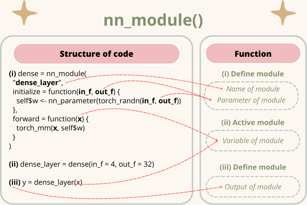
[ CPUFloatType{6,1} ][ grad_fn = <SliceBackward0> ]Module là 1 khái niệm quan trọng khi bạn làm việc tới package torch và đúng như cái tên của nó, module dùng để chứa 1 hoặc nhiều phép tính hoặc bao gồm cả module khác (hay còn gọi là submodule). Ví dụ như mô hình bên dưới mình đã tự xây dựng module cho mask self-attention và bao gồm nó bên trong module của decoder block.
Khi dùng hàm nn_module(), ta cần define 2 phần:
initialize: dùng để define các parameters hoặc submodule cần thiết để module hoạt động.
forward: dùng để define cách tính toán của module và sẽ hoạt động theo chiều bắt đầu từ trên xuống.
Mình cũng vẽ thêm biểu đồ này để mọi người dễ hiểu cách hoạt động của module.
Tiếp theo, mình sẽ xây dựng mô hình Transformer để dự báo giá cổ phiếu của Google từ nguồn Yahoo Finance.
#### Call packages-------------------------------------------------------------
pacman::p_load(quantmod,
               torch,
               dplyr,
               dygraphs)
#### Input---------------------------------------------------------------------
getSymbols("GOOG", src = "yahoo", from = "2020-01-01", to = "2022-01-01")
[1] "GOOG"price_data <- GOOG$GOOG.Close
price_data_xts <- xts(price_data,
order.by = index(price_data))
colors<-RColorBrewer::brewer.pal(9, "Blues")[c(4, 6, 8)]
dygraph(price_data_xts, main = "Google Stock Price (2020 - 2022)", ylab = "Price ($)") |>
dyRangeSelector(height = 20) |>
dyOptions(
fillGraph = TRUE,
colors = colors,
strokeWidth = 2,
gridLineColor = "gray",
gridLineWidth = 0.5,
drawPoints = TRUE,
pointSize = 4,
pointShape = "diamond"
) |>
dyLegend(show = "follow") Như biểu đồ, ta thấy giá cổ phiếu tăng cao chóng mặt và mức biến động khá mức tạp (lúc lên lúc xuống). Task này khá khó nên ta sẽ tìm hiểu xem performance của mô hình Transformer sẽ như thế nào.
Mô hình đầy đủ sẽ được code như sau:
#### Transform input----------------------------------------------------------------
create_supervised_data <- function(series, n) {
  series <- as.vector(series)
  data <- data.frame(series)

  for (i in 1:n) {
    lagged_column <- lag(series, i)
    data <- cbind(data, lagged_column)
  }

  colnames(data) <- c('t',paste0('t', 1:n))

  data <- na.omit(data)

  return(data)
}

seq_leng <- 50
dim_model <- 32

supervised_data <- create_supervised_data(price_data, n = seq_leng)

supervised_data <- scale(supervised_data)


x_data <- torch_tensor(as.matrix(supervised_data[, 2:(seq_leng+1)]), dtype = torch_float())  # Features (lags)
y_data <- torch_tensor(as.matrix(supervised_data[, 1]), dtype = torch_float())    # Target

# Reshape x_data to match (batch_size, seq_leng, feature_size)
x_data <- x_data$view(c(nrow(x_data), seq_leng, 1))  # (batch_size, seq_leng, feature_size)
y_data <- y_data$view(c(nrow(y_data), 1, 1))

# Split the data into training and testing sets (80% for training, 20% for testing)
train_size <- round(0.8 * nrow(supervised_data))

x_train <- x_data[1:train_size, , drop = FALSE]
y_train <- y_data[1:train_size]

x_test <- x_data[(train_size + 1):nrow(supervised_data), , drop = FALSE]
y_test <- y_data[(train_size + 1):nrow(supervised_data)]

#### Build components of model----------------------------------------------------------------
### Positional encoding:
positional_encoding <- function(seq_leng, d_model, n = 10000) {
  if (missing(seq_leng) || missing(d_model)) {
    stop("'seq_leng' and 'd_model' must be provided.")
  }

  P <- matrix(0, nrow = seq_leng, ncol = d_model)

  for (k in 1:seq_leng) {
    for (i in 0:(d_model / 2 - 1)) {
      denominator <- n^(2 * i / d_model)
      P[k, 2 * i + 1] <- sin(k / denominator)
      P[k, 2 * i + 2] <- cos(k / denominator)
    }
  }

  return(P)
}

en_pe <- positional_encoding(x_data$size(2),dim_model, n = 10000)
de_pe <- positional_encoding(y_data$size(2),dim_model, n = 10000)

### Encoder block:
encoder_layer <- nn_module(
  "TransformerEncoderLayer",

  initialize = function(d_model, num_heads, d_ff) {

    # Multi-Head Attention
    self$multihead_attention <- nn_multihead_attention(embed_dim = d_model, num_heads = num_heads)

    # Feedforward Network (Fully Connected)
    self$feed_forward <- nn_sequential(
      nn_linear(d_model, d_ff),
      nn_relu(),
      nn_linear(d_ff, d_model)
    )

    self$layer_norm <- nn_layer_norm(d_model)

  },

  forward = function(x) {

    attn_output <- self$multihead_attention(x, x, x)
    x <- x + attn_output[[1]]
    x <- self$layer_norm(x)

    # Feedforward network with residual connection
    ff_output <- self$feed_forward(x)
    x <- x + ff_output
    x <- self$layer_norm(x)

    return(x)
  }
)

### Mask function:
mask_self_attention <- nn_module(
  initialize = function(embed_dim, num_heads) {
    self$embed_dim <- embed_dim
    self$num_heads <- num_heads
    self$head_dim <- embed_dim / num_heads

    # Ensure that self$head_dim is a scalar
    if (self$head_dim %% 1 != 0) {
      stop("embed_dim must be divisible by num_heads")
    }

    if (embed_dim %% num_heads != 0) {
      stop("embed_dim must be divisible by num_heads")
    }

    # Linear layers for Q, K, V
    self$query <- nn_linear(embed_dim, embed_dim, bias = FALSE)
    self$key <- nn_linear(embed_dim, embed_dim, bias = FALSE)
    self$value <- nn_linear(embed_dim, embed_dim, bias = FALSE)

    # Final linear layer after concatenating heads
    self$out <- nn_linear(embed_dim, embed_dim, bias = FALSE)

  },

  forward = function(x) {
    batch_size <- x$size(1)
    seq_leng <- x$size(2)

    # Linear projections for Q, K, V
    Q <- self$query(x)  # (batch_size, seq_leng, embed_dim)
    K <- self$key(x)
    V <- self$value(x)

    # Reshape to separate heads: (batch_size, num_heads, seq_leng, head_dim)
    Q <- Q$view(c(batch_size, seq_leng, self$num_heads, self$head_dim))$transpose(2, 3)
    K <- K$view(c(batch_size, seq_leng, self$num_heads, self$head_dim))$transpose(2, 3)
    V <- V$view(c(batch_size, seq_leng, self$num_heads, self$head_dim))$transpose(2, 3)

    # Compute attention scores
    d_k <- self$head_dim
    attention_scores <- torch_matmul(Q, torch_transpose(K, -1, -2)) / sqrt(d_k)

    # Apply mask if provided
    mask <- torch_tril(torch_ones(c(seq_leng, seq_leng)))

    if (!is.null(mask)) {

      masked_attention_scores <- attention_scores$masked_fill(mask == 0, -Inf)

    } else {
      print("Warning: No mask provided")
    }

    # Compute attention weights
    weights <- nnf_softmax(masked_attention_scores, dim = -1)

    # Apply weights to V
    attn_output <- torch_matmul(weights, V)  # (batch_size, num_heads, seq_leng, head_dim)


    attn_output <- attn_output$transpose(2, 3)$contiguous()$view(c(batch_size, seq_leng, self$embed_dim))


    output <- self$out(attn_output)
    return(output)
  }
)

### Cross attention:
cross_attention <- nn_module(
  initialize = function(embed_dim, num_heads) {
    self$embed_dim <- embed_dim
    self$num_heads <- num_heads
    self$head_dim <- embed_dim / num_heads

    if (self$head_dim %% 1 != 0) {
      stop("embed_dim must be divisible by num_heads")
    }

    self$query <- nn_linear(embed_dim, embed_dim, bias = FALSE)
    self$key <- nn_linear(embed_dim, embed_dim, bias = FALSE)
    self$value <- nn_linear(embed_dim, embed_dim, bias = FALSE)
    self$out <- nn_linear(embed_dim, embed_dim, bias = FALSE)
  },

  forward = function(decoder_input, encoder_output, mask = NULL) {
    batch_size <- decoder_input$size(1)
    seq_leng_dec <- decoder_input$size(2)
    seq_leng_enc <- encoder_output$size(2)

    Q <- self$query(decoder_input)
    K <- self$key(encoder_output)
    V <- self$value(encoder_output)

    Q <- Q$view(c(batch_size, seq_leng_dec, self$num_heads, self$head_dim))$transpose(2, 3)
    K <- K$view(c(batch_size, seq_leng_enc, self$num_heads, self$head_dim))$transpose(2, 3)
    V <- V$view(c(batch_size, seq_leng_enc, self$num_heads, self$head_dim))$transpose(2, 3)

    d_k <- self$head_dim
    attention_scores <- torch_matmul(Q, torch_transpose(K, -1, -2)) / sqrt(d_k)

    weights <- nnf_softmax(attention_scores, dim = -1)

    attn_output <- torch_matmul(weights, V)

    attn_output <- attn_output$transpose(2, 3)$contiguous()$view(c(batch_size, seq_leng_dec, self$embed_dim))

    output <- self$out(attn_output)
    return(output)
  }
)

### Decoder Layer
decoder_layer <- nn_module(
  "TransformerDecoderLayer",

  initialize = function(d_model, num_heads, d_ff) {
    self$mask_self_attention <- mask_self_attention(embed_dim = d_model, num_heads = num_heads)
    self$cross_attention <- cross_attention(embed_dim = d_model, num_heads = num_heads)
    self$feed_forward <- nn_sequential(
      nn_linear(d_model, d_ff),
      nn_relu(),
      nn_linear(d_ff, d_model)
    )

    self$layer_norm <- nn_layer_norm(d_model)
  },

  forward = function(x, encoder_output) {
    # Masked Self-Attention
    mask_output <- self$mask_self_attention(x)
    x <- x + mask_output
    x <- self$layer_norm(x)

    # Encoder-Decoder Multi-Head Attention
    cross_output <- self$cross_attention(x, encoder_output)
    x <- x + cross_output
    x <- self$layer_norm(x)

    # Feedforward Network
    ff_output <- self$feed_forward(x)
    x <- x + ff_output
    x <- self$layer_norm(x)

    return(x)
  }
)

### Final transformer model:
transformer <- nn_module(
  "Transformer",

  initialize = function(d_model, seq_leng, num_heads, d_ff, num_encoder_layers, num_decoder_layers) {
    self$d_model <- d_model
    self$num_heads <- num_heads
    self$d_ff <- d_ff
    self$num_encoder_layers <- num_encoder_layers
    self$num_decoder_layers <- num_decoder_layers
    self$seq_leng <- seq_leng
    self$en_pe <- en_pe
    self$de_pe <- de_pe

    # Encoder layers
    self$encoder_layers <- nn_module_list(
      lapply(1:num_encoder_layers, function(i) {
        encoder_layer(d_model, num_heads, d_ff)
      })
    )

    # Decoder layers
    self$decoder_layers <- nn_module_list(
      lapply(1:num_decoder_layers, function(i) {
        decoder_layer(d_model, num_heads, d_ff)
      })
    )

    # Final output layer
    self$output_layer <- nn_linear(d_model, 1)  # Output layer to predict a single value

  },

  forward = function(src, trg) {

    src <- src + self$en_pe
    trg <- trg + self$de_pe

    # Encoder forward pass
    encoder_output <- src
    for (i in 1:self$num_encoder_layers) {
      encoder_output <- self$encoder_layers[[i]](encoder_output)
    }

    # Decoder forward pass
    decoder_output <- trg
    for (i in 1:self$num_decoder_layers) {
      decoder_output <- self$decoder_layers[[i]](decoder_output, encoder_output)
    }

    # Apply final output layer
    output <- self$output_layer(decoder_output)

    return(output)
  }
)

#### Training----------------------------------------------------------------
model <- transformer(
  d_model = dim_model,         # Embedding dimension
  seq_leng = seq_leng,        # Sequence length
  num_heads = 8,        # Number of heads
  d_ff = seq_leng,           # Dimension of the feedforward layer
  num_encoder_layers = 6,
  num_decoder_layers = 6
)


#### Training----------------------------------------------------------------
epochs <- 200
loss_fn <- nn_mse_loss()
optimizer <- optim_adam(model$parameters, lr = 1e-3)

for (epoch in 1:epochs) {
  model$train()
  optimizer$zero_grad()

  # Forward pass
  y_train_pred <- model(x_train, y_train)

  # Compute the loss
  loss <- loss_fn(y_train_pred, y_train)

  # Backpropagation and optimization
  loss$backward()
  optimizer$step()

  if (epoch %% 10 == 0) {
    cat("Epoch: ", epoch, " Loss: ", loss$item(), "\n")
  }
}

#### Predictions----------------------------------------------------------------
model$eval()

# Make predictions on the test data
y_test_pred <- model(x_test, y_test)  # Use the test data for both input and output during prediction

# Convert tensors to numeric values for comparison

y_test_pred<- as.numeric(as.array(y_test_pred$cpu()))

#### Evaluating----------------------------------------------------------------
library(highcharter)
y_train_pred <- as.numeric(as.array(y_train_pred$cpu()))
y_train <- as.numeric(as.array(y_train$cpu()))
y_test <- as.numeric(as.array(y_test$cpu()))

comparison <- data.frame(
  time = 1:nrow(supervised_data),
  actual = c(y_train,y_test),
  forecast = c(y_train_pred,y_test_pred)
)

# Compare only errors:
error<-highchart() |>
  hc_title(text = "Evaluating error of model") |>
  hc_xAxis(
    categories = time,
    title = list(text = "Time")
  ) |>
  hc_yAxis(
    title = list(text = "Value"),
    plotLines = list(list(
      value = 0,
      width = 1,
      color = "gray"
    ))
  ) |>
  hc_add_series(
    name = "Error",
    data = (y_test_pred - y_test)/y_test,
    type = "line",
    color = "red"  # Blue color for actual data
  ) |>
  hc_tooltip(
    shared = TRUE,
    crosshairs = TRUE
  ) |>
  hc_legend(
    enabled = TRUE
  )


# Compare all:
all<-highchart() |>
  hc_title(text = "Model Predictions vs Actual Values") |>
  hc_xAxis(
    categories = time,
    title = list(text = "Time")
  ) |>
  hc_yAxis(
    title = list(text = "Value"),
    plotLines = list(list(
      value = 0,
      width = 1,
      color = "gray"
    ))
  ) |>
  hc_add_series(
    name = "Actual Data",
    data = comparison$actual,
    type = "line",
    color = "#1f77b4"  # Blue color for actual data
  ) |>
  hc_add_series(
    name = "Forecast",
    data = comparison$forecast,
    type = "line",
    color = "#ff7f0e"  # Orange color for forecast data
  ) |>
  hc_tooltip(
    shared = TRUE,
    crosshairs = TRUE
  ) |>
  hc_legend(
    enabled = TRUE
)Đầu tiên ta sẽ đánh giá về sai số của mô hình khi dùng testing data. Kết quả khá ổn khi sai số khoảng (0.04,0.12).
Và còn nhìn tổng quan hết thì ta thấy mô hình dự đoán khá sát với training data nhưng với testing data thì vẫn chênh lệch thấp hơn thực tế (dấu hiệu cho thấy mô hình đang bị overfitting).
Như vậy ta đã thấy được sức mạnh của mô hình Transformer trong dự báo cho dữ liệu sequence (mặc dù mình mong muốn error rate < 0.05 nhưng kết quả vẫn chấp nhận được).
Một số suggestion của mình cho mô hình Transformer để improve performance như sau:
Thêm layer nn_dropout(p) vào mô hình: là một phương pháp regularization (chuẩn hóa) được sử dụng trong mạng nơ-ron để ngăn ngừa hiện tượng overfitting (quá khớp) bằng cách ngẫu nhiên “loại bỏ” một tỷ lệ phần trăm nơ-ron trong quá trình huấn luyện. Bạn chỉ cần thêm đối số p là tỷ lệ % dropout.
Dùng các variant của Transformer: thực chất mục đích ban đầu của Transformer là deal với các tasks liên quan về dịch thuật, xử lí văn bản, phân tích hình ảnh,… chứ không thiên về time series forecasting. Mô hình deep learning khác thiên về vấn đề này mà bạn có thể sử dụng là Informer.
Nếu bạn có câu hỏi hay thắc mắc nào, đừng ngần ngại liên hệ với mình qua Gmail. Bên cạnh đó, nếu bạn muốn xem lại các bài viết trước đây của mình, hãy nhấn vào hai nút dưới đây để truy cập trang Rpubs hoặc mã nguồn trên Github. Rất vui được đồng hành cùng bạn, hẹn gặp lại! 😄😄😄